When show a Carbonist that there is no evidence of CO2 causing significant “global” warming at any scale from deep time to the last 35 years as we did in the last post, they usually look at you funny and say, “Hey man, it’s a greenhouse gas, how can it possibly not cause warming?”

It is a very reasonable question. The answer can be found in the text speak of the title, and will be developed below.

Thanks to the cold war and the clear need to understand the spectral properties of the atmosphere for targeting and guidance systems, we have extensive laboratory work and computer code on atmospheric spectra and three levels of computer models meticulously calibrated by aircraft, balloon, and satellite to ground measurements. Much of this work was done at the Air Force Cambridge Research Laboratory at Hanscom Air Force Base.

Unlike the climate models currently undergoing first order calibration, the HITRAN, MODTRAN, and LOWTRAN models are mature and have undergone four decades of ever more accurate development. The following is from chapter 18 (Fenn et al, 1985) in  the Handbook of Geophysics.

It shows what the IRIS spectrometer on Nimbus 3 at 1100 km saw looking down. It also shows their calibration process. Below is a radiance spectrum by the same instrument class from Nimbus 4 at a similar altitude over the Sahara. This cartoon also shows the Planck temperatures that match the spectrum and the lapse rate of the atmosphere with possible altitudes that match the Planck temperatures. It also shows the “atmospheric window” where only the ragged and weak water bands and the shark bite of ozone mar a perfect Planck curve.

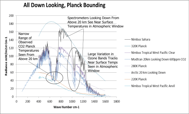
We need some lower altitude readings to limit the possibilities. The information is unavailable to the common man, or at least the exact aircraft and instruments used are hard to find. The Air Force had a number of planes that routinely flew at 20 km. There is a widely available spectrum looking down from 20 km meters and simultaneously up from the Arctic. We will explore that later, but it is hardly the place to go for a typical spectrum. Fortunately, the information is embedded in their code, and we have the MODTRAN spectrum at 600 ppm CO2 from 20 km altitude below.

From 20 km it is crystal clear from the intercepts that all the signal is coming from the tropopause or lower stratosphere. The irradiance units in the MODTRAN output were transposed to radiance by this method. What is most interesting is what has changed and what has not. The MODTRAN is for a U.S. standard atmosphere and the Nimbus is over the Sahara. The ~35K difference may be a bit much for average temperature difference, or not, depending on time of day and season. A bit of lapse at 280K cannot be ruled out from the intercepts. The weak water bands in the atmospheric window show a lot less amplitude as well as cooling a lot from 1100 km over the Sahara to 20km over the U.S. This seems to an an interesting general difference between arid and more humid regions as we will see.

By far, the most important result of this exercise is that while all the  water and ozone bands (and the CO2 “wings” at 600 ppm) shift to a lower temperature, the bottom of the CO2 bands does not within the accuracy of this cartoon, and may even increase a bit.

Here we jump back up to Nimbus and add two spectra from the tropical West Pacific. (Real time science need not follow a straight path.) You see how this works. In the atmospheric window outside the ozone “bite” in clear skies the spectrometer sees pretty much surface temperature and that temperature changes from place to place. Even the ozone bite changes temperature which is very interesting because it suggests the absorption is taking place nearer the surface than the stratosphere. What never changes is the “flat” bottom temperature in the CO2 bands.

The spectrum from the top of a thundercloud anvil is also very interesting. What makes it so cool is we know exactly where that is. The reason thunderclouds form a flat “anvil” top is because they hit the inversion where warmer temperatures above prevent further rise. Didn’t want to clutter the graphic, but trust me, through the atmospheric window (now shut) except for the bumps in the CO2 and ozone bands, the temperature tracks the 215K Planck curve like it was on rails. That was the temperature of the cloud top that day and the CO2 and ozone bands were radiating at a higher temperature. This strange behavior foreshadows Antarctica as we will see.

We have been trying to follow a consistent line of reasoning. The problem with all prior analyses has been inconsistency. They switch units in mid stream, making real understanding very difficult. We have followed earth spectrum radiance from Nimbus level 1100 km to MODTRAN 20 km altitude with the same units. Below this level the data vanishes. Maybe it is classified? Maybe the troposphere is too noisy for the old instruments?

Anyway, there seems no choice but to switch units. The information for the troposphere is available in model form as “transmittance” and “absorption.” These are inverse (one minus the other) and expressed on a scale from zero to one. Before switching to a troposphere scale format transmittance at 280 ppm or pre industrial CO2 is added to the current platform below along with the ozone profile.

What is interesting is that the zero transmittance flatspot at pre industrial CO2 is broader than the “flat” bottoms all the satellite and MODTRAN radiance spectra show at 217 K, and the “arms” of 280 ppm transmittance are broader than even the 600 ppm MODTRAN radiance.

We have shown that all the measurements and model looking down from above the tropopause see photons in the CO2 bands radiating at the temperature of the lower stratosphere. We have established that a virtual spectrometer flying just below the tropopause and looking down (as represented by model transmission) sees nothing in a somewhat broadened “flat spot” in the same bands. Zero transmission.

Somewhere between the surface and the tropopause the 2 good greenhouse gas has gobbled up all those photons. We will explore this and start “looking up” at troposphere scale in the next post.