
We know the position and velocity of stable points on our six cratons. A reasonable question to ask is, “Can we account for this motion?”
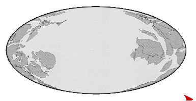
Above is a map of the ocean floor created in the last 10 million years. We will start at the present and work backwards, as 100% of the ocean floor is available to aid our constraints.
The present ocean floor is 361 million square kilometers. This map shows 27 million square kilometers, or ~7.5% of the current ocean floor extruded in the last 10 million years.
Of the last 10my extrusion, nearly 12 million square kilometers, or ~44%, was extruded by the East Pacific Ridge, shown in magenta. The Nazca, shown in rose, extending toward Chile, and the Juan de Fuca shown in lighter magenta off the Pacific Northwest add another ~1.4 million square kilometers.
A careful examination of the isochrons around the prominent “arm” of the Pacific ridge pointing towards Panama, and the Nazca arm as well, shows that even these exerted spreading force according with the predominant east-west axis of the ridge.
Very nearly 50% of the ocean floor extruded in the last 10 million years has been in the Pacific Ocean basin. The Americas are poorly connected to the Pacific basin and have continued moving westward even as the spreading ridge has moved eastward. The Pacific basin has been subducted beneath the advancing Americas. Whatever braking effect this subduction may have had, half of the ocean spreading in the last 10 million years cannot be used to constrain the motion of the Americas.

There is currently little or no subduction going on around Antarctica. The Australian-Antarctic ridge in rose and the Pacific ridge join in a peculiar fashion. In a 2013 post we discussed the oddity that Antarctica is circumscribed with ridges, yet has no trenches. Antarctica has moved about 135 kilometers and rotated about 3 degrees as shown. This Antarctic motion is about 50% more that the spreading of the Atlantic and Indian ridges apparently pushing the right direction, and is less than half of the antagonistic spreading of the Pacific and Austral-Antarctic ridges.
In order for this motion and growth to be accomplished without expanding the earth, the entire system must have moved with Antarctica. The motion of Australia is ~28% greater than the combined spreading of the ridge and motion of Antarctica.

Africa is also caught between spreading ridges with little or no current subduction. It has moved only about 40km west to east at its 58 degree bearing. The motion of South America is in reasonable agreement with the spreading of the Atlantic ridge.

It would be truly astonishing, and call into question our most fundamental concepts of plate tectonics, if the motions of North America and South America could not be accounted for by the spreading of the Atlantic ridge. The pieces fit together like a puzzle, existing magnetic lineations cover the entire interval since separation, and the existing ridge tracks the shapes.
We can see that the motions do generally conform to the scale of Atlantic spreading over the last 10 million years. What remains to be explained is why Africa and Eurasia remained relatively fixed in longitude while the ridge and the Americas moved to the west.
There are two areas in the mantle with the chewy name of LLSVP’s where shear waves are attenuated. I call these Low Velocity Provinces doughboys. They appear to be extrusions from the core. One is under Africa, and the other out in the Pacific. Their footprints at the core-mantle boundary (the bottom of the box) are at the 1% anomaly contour and all sorts of plumes and kimberlite pipes seem to originate there as suggested in the upper panel and red dots at the surface.

Above we have plotted the 1% footprints of the doughboys (after Torsvik). These footprints are thought to have remained fixed in relation to the core. Their highest reaches flatten out at the 660km discontinuity, and the crust has moved around above them. It seems possible that Africa is somehow grounded in its doughboy, and being substantially connected to Eurasia for the last 10 million years, has restrained this entire mass while the Americas moved to the west.
We have the extrusions of the Greenland Ridge, seemingly an extension of the Atlantic ridge; and the Lomonosov ridge, nearly crossing the North Pole, to complete our 0-10mya analysis. These ridges seem to be in accordance with the very modest SE motion of Eurasia and the bearing of North America ~15 degrees south of due west. Once again, with no trenches, the Arctic spreading ridges must have moved away from Eurasia their spreading distance less the 49km opposite motion of Eurasia.
The answer to the question at the beginning of this post, “Can we account for this motion?”, is ambiguous. We can account for the motions of the Americas, Eurasia, and Africa; with the caveat that the explanation for the relative fixation of Africa and Eurasia is hypothetical. The motions of the Austral pair, Antarctica and Australia, are wildly out of scale with adjacent spreading. As the ridges must necessarily have moved with Antarctica, we must conclude that the motions of Antarctica and Australia remain unconstrained.
It seems far too tedious at this point to step back 25 times through our 10my increments. In the next posts, we will focus on the inflection points.


