MODTRAN, The One ppm Exercise

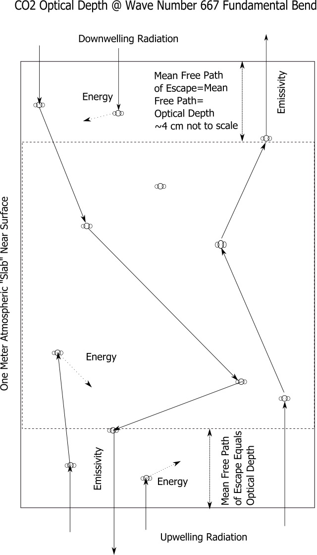
MODTRAN is impressively nuanced sometimes. Ordinarily MODTRAN is used on a macro scale at plausible altitudes and greenhouse gas concentrations, but it definitely resolves at single meters of altitude and single ppm of greenhouse gasses.

Here we explore one ppm CO2 with all the other GHG’s zeroed out. We look both up and down from one meter, and 70 kilometers.

Modtran Up and Down 1 meter 1 ppm ann

Beginning at one meter, we see little difference from the Planck curve looking down. This is no different from what we see at 400 ppm looking down up to about 400 meters altitude, except that there is .31 W/m2 MORE upward radiation at 400 ppm.

Looking up from one meter the reach of a single ppm of CO2 is astonishing. The 667.4 fundamental bend does not quite kiss the downward looking curve, meaning that it is seen radiating from some small distance above one meter. Only the fundamental bend can be seen radiating from essentially the surface to an altitude of about six kilometers.

At the temperature of six kilometers the additional bending vibrations at 647.1 and 688.7 kick in, along with the P and R rotations dependent on the fundamental bend. At a temperature 15 kilometers we see the additional vibration at 618 and the bend to stretch transition at 720.8

Interestingly, at 1 ppm you get almost a “chromatograph” of the relative intensities, with the factor of progressive movement away from top dead center of the Planck curve with increasing altitude omitted.

Modtran up and down 1 ppm 70 km

The view of 1 ppm from 70 kilometers is I’m many ways the inverse of the view from one meter. Looking up from 70 km there is essentially no IR coming down from above. Looking down we see the “effective radiative levels” of the CO2 transitions to space. The fundamental bend at 667.4 is seen radiating at a temperature of 12 km, and once again it shows extraordinary reach, being the only signal from 6 to 12 kilometers.

At 1 ppm, there is essentially no difference in either upward or downward radiation above 25 km elevation.

Just for kicks, below is 1 meter looking up vs 70 km looking down at 1ppm.

One meter looking up vs 70 km looking down

Let’s compare the 1 meter up and down view at 400 ppm.

Looking down, there is no discernable difference from 1 ppm, and the total upward IR flux is only .31 W/m2 more at 400 ppm.

There are lots of differences looking up. The fundamental bend and rotations, and the nearby three order of magnitude weaker transition at 647.1, have melded into a zone radiating at the Plank temperature of the ground (299.7 K). Notably, this is above the temperature seen looking down. The upwelling radiation deviates from the Planck curve more at top dead center than elsewhere along the curve. The downwelling radiation is seen at a higher temperature at the ground BB curve.

The transitions at 618 and 688.7 radiate at about the upwelling (down looking) curve, 597.3 and 720.8 are seen radiating at the temperature of perhaps 800 meters, and a crop of extremely weak transitions is seen radiating above 9 kilometers.

Astonishingly, there is a 60.5 W/m2 increase of downward flux between 1 ppm and 400 ppm, as seen from one meter elevation.

Here is 400 ppm up and down from 70 km.

Up and Down 70 km annotated

We have the usual cast of transitions, but their intensities (and temperatures) change with altitude and CO2 concentration. The difference in upwelling radiation between 1 meter and 70 km is 118.75 W/m2 at 400 ppm.

A transition can be deemed “saturated” when it radiates at a temperature conforming to the Planck curve. At 400 ppm from 70 km, the fundamental bend rotations are radiating at the 220K (12 km) curve, but the 667.4 bend itself reaches back down to a temperature of 9 km.

For kicks again, 1 meter looking up vs 70 km looking down at 400 ppm.

One meter looking up vs 70 km looking down 400 ppm


The fundamental bend is saturated looking up from a meter, but not above 9 km in the atmosphere.

Posted in MODTRAN | Tagged | Leave a comment

Infinity and Things to Do.

Infinity is meaningless. Everything is nothing.

When you rise every morning, the possibilities are infinite.

The difference between everything and nothing is you.

Posted in Climate | Leave a comment

Alexa and Chatty Cathy

Chatty Cathy was a doll. You could pull this string on her and she would say something random. She was the first electronic fortune cookie. She could say  maybe a dozen and a half different things. Never anything cogent. Some tangy things to keep your interest, some sweet things to butter you up, but nothing to piss you off by design.

So it is with Alexa. Algorithm rather than string. Marketing to lonely people. A pretense that your voice phonons in a virtual world, in  conversation with a remote server, is real.

Handy, but not real. Handy as a voice activated search engine (there are others). Handy if you want to listen and nobody else wants to talk…

Posted in Human need for Judgdment, Sociology | Leave a comment

The Terribly Tenacious Trough


Humans are prone to emotional conclusions like “the weather has gone crazy”. Last year at this time, even with the normal rainfall in the north half of the state, many asserted that California was in “new normal” permanent drought. The far above normal rainfall throughout the state this year shows that this sentiment is clearly wrong, but the same folks who set forth permanent drought will now assert unprecedented “crazy rain”.

We have done a series of posts on the drought in California using data from San Francisco that dates back to 1850. Here we present a look at the same data looking at high rainfall years in the same data set to evaluate how crazy this year really is.

SF Cumulative 2016-17

Perhaps this year’s trough is not so terribly tenacious after all. The season is not over and the tingling in my own bones is that it will be a wet spring, like many I remember from the seventies. Nevertheless, if I were a betting man, I would bet that this year will top out below the five previous years shown. If this season dries out, there will be more years to add above this year.

The point here is that the “ridiculously resilient ridge” that led to four consecutive years of below normal rainfall in California did not produce any individual years of record drought. If the terribly tenacious trough does the same in reverse, where are we?

As we have always been; naked apes staring into the sunrise. Is God punishing us?

If you want to project your guilt onto statistical noise, you go.

I’m going with the data.

Posted in Climate | 1 Comment

Effective Radiative Level

There is this concept that by averaging all the different radiative spectra that satellites see from earth from very high altitudes an Effective Radiative Level can be derived that has meaning for the radiation balance for the planet.

The basic idea is that the addition of greenhouse gasses, predominantly CO2 by humans, will raise the Effective Radiative Level. The further idea is that this supposed increase in altitude for the radiative level takes place within the part of the atmosphere where there is lapse, i.e. the atmosphere cools with increasing altitude.

The claim is that since a higher altitude implies a cooler temperature, the radiation to space will take place at a lower blackbody temperature with lower energy to the fourth power, and will cool the planet less effectively.

We have developed the tools to evaluate this claim. Rather than a single average level and blackbody temperature, the satellites see substantial differences in radiative altitude across the earth longwave spectrum.

All Down Looking, Planck Bounding

The “effective” radiation seen from space in the earth long wave spectrum ranges about 100K, from a remarkably consistent  220+-7K for the CO2 bands to a wildly different 320K+ in the atmospheric window.

The bottom line is that CO2 has its own radiative channel to space entirely separate from the effective Planck temperature of the atmosphere as a whole. This channel radiates at the tropopause and above where the lapse rate reverses and becomes negative. Rather than radiating at a lower temperature, with increasing concentration and higher radiative altitude, CO2 radiates to space to the fourth power of a higher temperature with increasing concentration.


Posted in Climate | Leave a comment

The Apology of Chaos

One grows weary of the, “it’s a non-linear, chaotic system” apology for human failing to accurately model weather and climate. This idea seems to have stunted roots in the very different worlds of the Lorenz Butterfly, and quantum probability.

Never mind that the scales of these two worlds are wildly different, and what may be currently unknowable at quantum scale is definitely not unknowable at butterfly scale.

The logical extent of this conflation of concepts leads to the conclusion that by merely observing Lorenz’ butterfly, we disturb it and irretrievably alter the future.

In the real world the effect of a butterfly wing flap is as insignificant to weather and climate, as quantum wave function probability is to navigating to the moon.

Chaos becomes an apology, an excuse to throw up ones hands and declare the task impossible. The task of understanding weather and climate is not impossible. It is just very difficult.

Posted in Climate | Leave a comment

Alternate “Facts” and Science.

Every “fact” so far that we naked apes have ever believed we have known, has proven to be incorrect at some level.

The operative verb in the sentence above is “believe”.

Alternate facts discovered by inquisitive people challenge the existing system of belief.

Often, when there is no clear economic benefit from the challenging fact, the investigators are persecuted.

Human nature.

[metalogue]: Science is the business of discovering alternate facts.

Posted in Climate | Leave a comment

Einstein and Weight Loss

Weird idea of the day: why your excessive butt or belly is so unresponsive to exercise, but so responsive to how much you eat.

Of course it is the equation. He won the Nobel Prize for something else, but the famous three term equation rings like a common field through separate universes from weight loss to particle physics.

The equation is pretty intuitive compared to most mathematical hieroglyphics, but I’m going to write it in English anyway.

Energy (what you eat)=mass (your butt) times the speed of light squared. Needless to say, the speed of light is a really big number to start with. When you square it, it gets completely out of hand.

Pretty simple. When you eat more energy than your body consumes, your butt (or belly) grows at the speed of light squared.

We all have our little indiscretions. It tastes sooo good. To get that excess mass off your butt, you must set the treadmill to the speed of light squared.

Simple (wink).


Posted in Chaos, Climate | 3 Comments

Emissivity of CO2

There is a lot of confusion about emissivity. Emissivity is the tendency to emit; particularly the tendency to emit light after absorbing it. In the infrared part of the spectrum, where the earth emits radiation towards the atmosphere, there is very little scattering. Incident light is either absorbed, or it passes through.

absorbance-transmission-emission

It can be seen that the light transmitted is equal to the light that passes unhindered plus the light that is emitted after absorption. The rectangle above can be thought of as a slab of atmosphere.  Transmission is the incident light minus the transmitted light. Transmissivity is the transmitted light divided by the incident light. Emissivity is the proportion of light emitted to the light absorbed.  For a perfect blackbody, emissivity is 1.

CO2 is far from a perfect blackbody.

Hottel and Leckner measured the column emissivity of CO2 in the 1940’s and 1970’s, respectively, at .14. Nasif Nahle has calculated a much smaller emissivity, .002, using two different methods. Staley and Jurica (1972) get .19. The range seems to be between poor and spectacularly poor emissivity, .002 to .2.

It turns out that in either case, the extremely high (98% in one meter) absorption of CO2 at 15 microns/wave number 667.4, and the poor transmission (2%), renders emissivity unimportant as regards upward radiation. The range of emissivity simply bounds the amount of light that passes straight through without being absorbed.

PQR2

Above is the one meter absorption of CO2 at 400 ppm. The Q branch at 667 is 98% absorbed in one meter. This means that only 2% is transmitted. This transmission includes both absorbed and re-emitted light and unhindered light passing straight through.

Where emissivity becomes important is back radiation, as an equal amount to what is absorbed and re-radiated up, must be re-radiated downwards as well. The highest published full column emissivity is ~20%. This would seem to be the high limit of full column back radiation.

What about individual layers?

Staley and Jurica give a value of .08 for CO2 emissivity of a slab of one centimeter optical depth, a value of .14 for 10 centimeters, and a value of .19 for a meter. Optical depth is defined in several different ways by astronomers, chemists, and atmospheric scientists. Astronomers treat optical depth as the mean free path through a slab. In this treatment “mean free path”, “path length”, the distance a photon travels after entering before interaction, the average distance between interactions, the distance between the final interaction and escape, the distance you can “see” into the material, and optical depth; are essentially the same.

Optical depth is also defined as the path length times the absorption coefficient. The one meter absorption coefficient for the CO2 fundamental bend is .98.  Path length is defined as partial pressure times the layer thickness. If the layer thickness is one meter, and the partial pressure is .04, the path length also becomes .04. We multiply this by the absorption coefficient to get an optical depth .04*.98*100(centimeters of CoE to a meter)=3.9

Beer’s Law defines optical depth as the negative natural log of transmittance. This is one of those mysterious empirical fits that work with surprising frequency. Transmittance is one minus whatever doesn’t get through (absorptance), so the negative natural log for a meter layer thickness and therefore the optical depth is -Ln(.02)=3.9. What luck.

The difference between the astronomical approach to optical depth and the chemistry and physics approach is that for astronomers optical depth is an actual distance, while the physical/chemical optical depth is dimensionless.

transmission-emission-pass-through


We can do a sanity check above where we plot linear values through a one meter slab by projecting centimeter scale values from measurements and calculations (.02 transmission, .08 emissivity/cm optical depth) We know perfectly well that none of this is linear, but transmission, and transmission minus emission are virtually indistinguishable. What this crude exercise can tell us is that it is very unlikely that any 667.4 photons pass through a one meter slab of atmosphere at current CO2 concentration. What we see transmitted through the slab is absorbed and re-emitted.

We can therefore assume that transmission, emission, and back radiation are all equal.

Back radiation must run the gauntlet of CO2 molecules on its way down as well. What we see radiated back down has the same mean free path to escape as what is transmitted up.

optical-depth

While the optical depth and free path remains the same up and down, the number of photons absorbed coming up, compared with those re-emitted in either direction, is reduced by the factor of emissivity. Back (downwelling) radiation can be no more than 2% of upwelling radiation.

The Schwarzschild equation used in radiative transfer models gets this completely backwards. The logic of this equation includes a “sink function” for absorption and a “source function” for re-radiation.  This “source function” is given as the absorption coefficient, .98 in this case.

This would be true according to Kirchhoff’s Law  if CO2 was a good blackbody with an emissivity of 1. We have seen that CO2 is a lousy blackbody with full column emissivity somewhere between .002 and .2. The value we have developed above, .02, falls in this range.

The “source function” in the Schwarzschild equation must be very significantly adjusted downward to reflect the real world emissivity of CO2.


Posted in Climate | 4 Comments

Berkeley Earth, The Arbitrary Use of Parameters to Create a Spurious Correlation

berkeley-earth-natural-log

Temperature, CO2, and volcano data | More recent data | High-resolution image The annual and decadal land surface temperature from the BerkeleyEarth average, compared to a linear combination of volcanic sulfate emissions and THE NATURAL LOGARITHM of CO2. It is observed that the large negative excursions in the early temperature records are likely to be explained by exceptional volcanic activity at this time. Similarly, the upward trend is likely to be an indication of anthropogenic changes. The grey area is the 95% confidence interval. (Capitals mine)

The graphic above has been widely used to establish a relationship between human CO2 and temperature. I was unable to replicate it. Stephen Mosher very kindly steered me towards a link on the Berkeley Earth site with an excel sheet.

Using their spreadsheet I first analyzed the components.

component-analysis-berkeley-earth

The volcanic correlation is interesting, but a very large negative temperature excursion in 1758 seems unsupported by major volcanism, and many temperature drops seem to have begun before the corresponding volcano.

There is certainly no important correlation (.46) between CO2 and the Land Only data. So I wanted to see how the correlation in the Berkeley Earth graphic was achieved. We are given an equation for the “fit”: Fit = alpha + beta * log( CO2 / 277.3 ) + gamma * Volcanic. The values of the parameters are given as:

alpha:  8.342105
beta:  4.466369
gamma:  -0.01515

It is well known that there is an approximately logarithmic diminution in transmission as CO2 in a jar is increased, so a logarithm is a reasonable place to look for getting CO2 in line with temperature.

berkeley-co2-logco2

You can see that the log of CO2 is no fun at all. It is way too flat. We are given the common log, not the natural log, so we take this as a error in the caption of the Berkeley graphic.

berkeley-alpha-log

I know, let’s add a parameter. We hear a lot about parameterization, but rarely get to see it in action. Here we step through the equation one term at a time.

berkeley-alphabeta

Hot damn! That’s a much better fit at the end, but there are some jagged toes on that foot.

berkeley-volcanic

And with the volcanic parameter the shoemakers have finished their fit.

I am not at all impressed with this process. The author states the rationale:

Because the RCP estimates that most forcing time series are highly correlated to CO2,

it follows that 98.5% of the variance in their total forcing curve can be mapped by just

CO2 and volcanism.

He started with a preconception based on Potsdam forcing data that the correlation must be close, and felt no qualms about using tunable parameters to create a spurious correlation.

True scientists don’t run in those shoes.

Posted in Climate | Leave a comment